Acceleration of Gravity Lab

We did this lab to serve to purposes: to determine the acceleration of gravity from a free falling object, and to gain experience using the computer software to collect data.

The materials needed for this lab are:

• a Lab Pro Interface
• Logger Pro Software on a computer
• Motion Detector
• rubber ball
• wire basket

In this lab we are trying to find the acceleration of gravity by measuring a the fall rubber ball with the motion detector hooked up to the Lab Pro Interface and collect the data onto Logger Pro where it will record it all. Logger Pro will also create a graph of both the velocity of the ball and the acceleration. We will look at these graphs to solve for the acceleration of gravity.

To begin this lab we loaded the Logger Pro software and opened the file, "graphlab", which contained the settings needed to run this lab. We are given a blank position vs. time graph which is where we will be collecting our data from. Set up the motion detector face up underneath the wire basket but in a space where none of the wires of the basket interfere with the motion detector. Also, make sure the motion detector is hooked up to the Lab Pro Interface, which also needs to be plugged into the computer's USB slot.
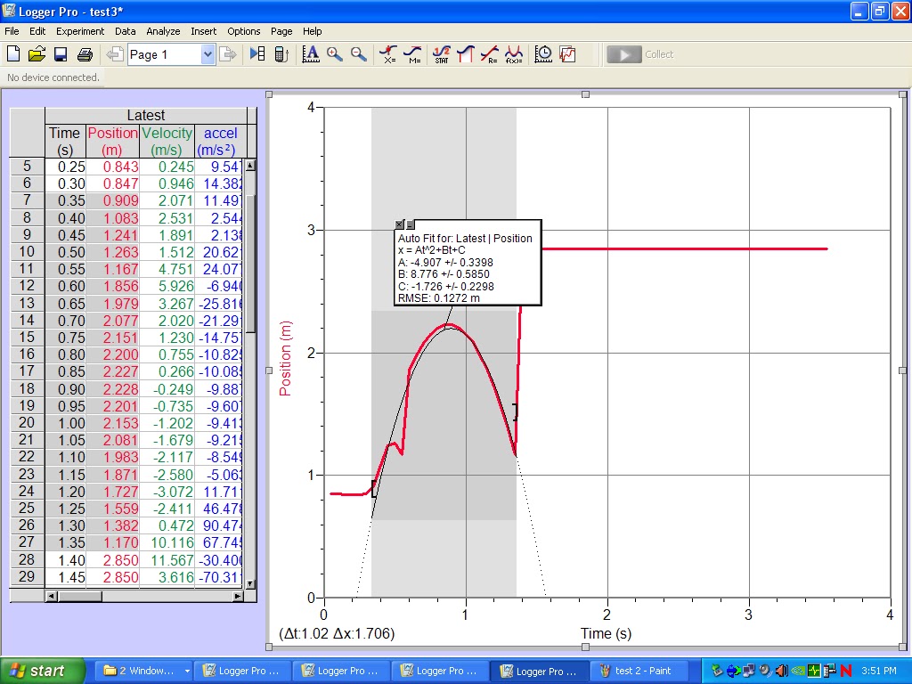
Once everything is hooked up and set, hit the "Collect" button, and throw the ball above the motion detector until it hits the ground and you see a position vs. time graph that has a negative quadratic parabola. We collected 5 of our best trials and saved their data. After we had the trials we wanted, we set a curve fit on all 5 position vs. time graphs to see what the equation would be that described the ball's motion of each trial. We solved for our experimental gravity for the trials (which is 2 times A, where A is the coefficient of the squared term of the equation given when you put on a curve fit) then solved for the percent error to show how close we were to solving for the accepted value for gravity, which is 9.8 (m/s)^2.
Change the y-axis label on the graph from position to velocity to show the velocity vs. time graph. Here, we want to find a part of the graph where there is a line to show a constant change in velocity with respect to time. Select the area that has the straightest line and select a linear fit in that portion of the graph. Do this to all 5 graphs and the slope, m, for all of these graphs should be close or equal to  -9.8 because the change in velocity describes acceleration. The constant change in velocity would show constant acceleration. Once solving for the value, m, calculate the % error and compare to your previous value for gravity.

CALCULATING PERCENT ERROR

percent error = |[(measured - actual)/actual]| X 100

DATA

This table shows our values of gravity compared to the accepted value for gravity as well as the percent error that occured for each graph.

GRAPHS 

TRIAL 1:

Position vs. Time

 

Velocity vs. Time

TRIAL 2:

Position vs. Time

Velocity vs. Time

TRIAL 3:
Position vs. Time

Velocity vs. Time

TRIAL 4:

Position vs. Time



Velocity vs. Time

TRIAL 5:
Position vs. Time

Velocity vs. Time



 

The graph of position is in the shape of a parabola because it is describing the distance of the ball from the motion detector. When the ball is first thrown, it's initial position is at about 1 m. Its height increases and time increases until it reaches it's highest point then it decreases in height falling at a faster pace the more time passes.

 

Each of these graphs all show the "A" value of their quadratic equations in the Position vs. Time graphs (in red). The slope, m, is given in the Velocity vs. Time graphs (in green) which describes the constant acceleration that occurs when the ball is thrown and is taken by gravity. The slope should be very close to -9.8 because that is acceleration of gravity.

 

The slope of the Velocity vs. Time graph represents the acceleration. When the velocity is positive it represents the increasing height of the ball. When it is equal to 0, this is when the ball reaches its heighest point and doesn't move for that split second. The negative velocity represents the ball falling from its highest point to when it hits the ground. The reason this graph is a line with a negative slope is because the as time increases, the slope of the position decreases from a positive slope to 0, then from 0 velocity down to a negative velocity.

Unit Analysis:

When we look at these graphs, we are given lots of information. When looking at the Position vs. Time Graphs for all of the trials you can see the equation of the fit that was performed. Looking at this equation we are given x=At^2+Bt+C where:

• A = acceleration.........................................(m/s^2)
• B = velocity................................................(m/s)
• C = position................................................(m)

You can solve for your experimental gravity by multiplying A by 2. It should be very close to if not -9.8 m/s^2. It is negative because gravity pulls things down which in mathematical terms means it is going in negative direction.

When looking at the graph of Velocity vs. Time we see something different. We see a line, not a parabola and instead of doing a curve fit we do a linear fit for this graph to find acceleration. Once performing a linear fit, you are given an equation v=mt+b where:

• m = acceleration...........................................(m/s^2)
• b = velocity..................................................(m/s)

We can use this graph to find our experimental gravity which in this case would be the m, or slope, of the velocity graph.

Conclusion:

In this lab, we looked at how to solve for the acceleration of gravity by tracking a falling ball and interpreting their Postion vs. Time graph as well as the Velocity vs. Time graph. I learned through the unit analysis, what each coefficient of quadratic and linear functions are and how they can help us solve for gravity. We were able to solve for the gravity from our results but they weren't all exactly the -9.80 m/s^2 we were trying to achieve. This is because of the errors that could have occured during lab like when we were throwing the ball there wasn't exactly a perfect scenario to make a perfect graph. Some things that could have possibly affected it was the motion detector not being able to follow the ball within 1 meter of it which made the graph do all the crazy spikes that occurred. That is why we ended up selecting a portion of the graph that was smooth and continuous to select a fit whether it was a curve fit or linear. There was also trial and error when throwing the ball up because we didn't get it perfectly above the motion sensor everytime and the motion detector was also covered by a wire basket that it could have picked up instead of the ball to throw our data off.