Vector Addition of Forces Lab

In this lab we studied vector addition by graphical means and also by using vector components. The materials to replicate this lab are as follows:

• Circular Force Table
• 4 pulleys
• Masses
• Mass Holders
• string
• Protractor and ruler

Intro:
Vectors are arrows with a certain length, which describes the magnitude of an object, and direction. In order to add vectors you must have the vector components which describe how far along the x and y axes the magnitude of the vector travel which will give you <i, j> where i is the x direction and j is the y direction. To find the components of a vector that gives you the magnitude as well as the angle of direction you would use basic trigonometry identities.

To find the x component:

cosӨ = V_x /M

McosӨ = V_x 

To find the y component:

sinӨ = V_y/M

MsinӨ = V_y

Once you find your vector components the notation of your vector you will have <V_x ,V_y >. When you have at least two components you can now add them together by adding the x components and the y components to get the components of the two added vectors which will make up a new vector that you can graph.

Another method you can use to add vectors is graphically.

In this picture you can see that in order to find V₃ you would draw it from the tail of the first vector which is V₁ to the head of the last vector which is V₂.

Procedure:
In this lab we are given 3 masses and an angle by our teacher. The 3 masses and angles we were given were:

• 150 g @ 0°
• 110 g @ 70°
• 250 g @ 135°

We were given a conversion to convert the masses into lengths for the magnitude of our given vectors. The conversion was 1cm = 20 g. We used the conversion and found the magnitudes of our vectors:

• 7.5 cm
• 5.5 cm
• 12.5 cm

We graphed the 3 vectors using the head to tail method first to find the magnitude and the direction of the angle.

We measured the length of the resulting vector with a ruler to be 14.0 cm and 87.75° with a protractor. 

Once we found the resulting vector using the graphic method we then solved for the resulting vector by finding the components of the given vectors.

With these components we were able to find the magnitude and angle of the resultant vector.

Data Analysis:

Now that we have a magnitude and direction for our new vector we now convert it to grams by using the conversion 1 cm = 20 g which gives us 280.4 grams for our resultant vector. We then set up our circular force table with the four pulleys. At the center there is a ring with 4 strings tied from it that hung off of the pulleys. The first 3 pulleys were set at the given angles, 0°, 70°, and 135°. The fourth was set 180° opposite the angle we found which was 87.8. This gave us a new angle 267.8° which now makes our vector negative. After having all of the pulleys set we then hooked the massholders to the ends of all of the strings and added the masses onto the massholders:

The center ring was in equilibrium on the circular force table which means the masses hanging at the end of the strings which hung from the pulleys at the correct angles suspended the ring in the center without touching anything.

We showed the direction of all the vectors to understand the direction they are going on the table.

Conclusion:

We calculated our percent error to be 0.14%. It was a low because we were able to control most of our experiment since we were only trying to find one vector from 3 vectors. The one that was more off was when we solved for it graphically only because we were physically measuring rather than working with the components. In this lab we learned how to add vectors by their components and also graphically with the head to tail method.



Acceleration of Gravity on an Inclined Plane Lab

The purpose of this lab is to find the acceleration of gravity by observing the motion of a cart on an inclined plane. In this lab we will be using:

• Logger Pro Software
• motion detector
• ballistic cart
• aluminum track
• woodblocks
• meterstick
• small carpenter level

Intro:
We will be using Logger Pro to collect the position vs. time data for the ballistic cart as it accelerates along the aluminum track. We are not going to include the effect of friction because friction will act with the force of gravity as the cart moves up the track and against gravity while it travels down the track. With this, we can use the average acceleration of the cart moving up and down the track with:

(a1+a2) / 2

to determine the average acceleration of gravity as the friction will slightly increase acceleration of gravity while the cart moves up the track and decrease slightly as the cart moves down the track. The average acceleration of the cart is equal to the acceleration due to gravity, g, times the sine of the angle of the track.

We can use this picture to find the acceleration of an object on an incline plane. We have θ because that is equal to the angle of the plane with the table. We also have the acceleration of the freefall and the acceleration of the object parallel with the inclined plane. If we look at them as vector components we see that we can add | a_parallel |+| a_{perpendicular} | = a_freefall

We see that g is the same as the a_freefall and can come up with the equation:

sinθ = opposite / hypotenuse

sinθ = | a_parallel | / g

Knowing this we can substitute in the average acceleration of the cart going up the track and going down the track:

| a_parallel | = (a1+a2) / 2

and we can arrange the previous equation:

sinθ = [(a1+a2)/2] / g

g sinθ = (a1+a2) / 2

and in order to find g, the acceleration due to gravity, we divide both sides by sinθ:

g = [(a1+a2)/2] / sinθ

where a1 and a2 are the accelerations of the cart, θ is the angle of the track and the table, and g is acceleration due to gravity.

Procedure:

First, we hooked up the Logger Pro software and opened up the graphlab file which is where we recorded all of our data. We then set up the aluminum track with one side having 1 wood block underneath its feet which raised up the track to give it an incline. Using the bubble level, we made sure the width of the track was level to make sure there wouldn't be any other effects of friction that could taint our results. After that we set the motion detector at the top of the track having it face the bottom part of track where the cart will be coming from that way we could measure its position, velocity, and acceleration.



Once having the lab set up we then solved to find the angle that θ would be by doing some simple trigonometry. We measured out 50 cm on the length of track and used the level to make marks on the table vertically below where the 0 cm were on the track and where 50 cm were on the track. We found that length to be 49.95 cm. Now, in order to find the measure of angle θ, we use the equation:

cosθ = adjacent side of the angle / hypotenuse

which, when using our measurments, comes to be:

cosθ = (49.95cm/50cm)

(arccos(cosθ)) = arccos(49.95/50)

θ = 2.56°

Before starting we opened up two graphs in Logger Pro, one of the position vs. time and one of the velocity vs. time to compare the two as they are occuring. We did a few practice trials to get ourselves comfortable trying the system out and making sure everything was going to work smooth for the lab. Once doing that, we did 3 trials of pushing the cart up the track and letting it come back down with the effects of gravity.

Results:

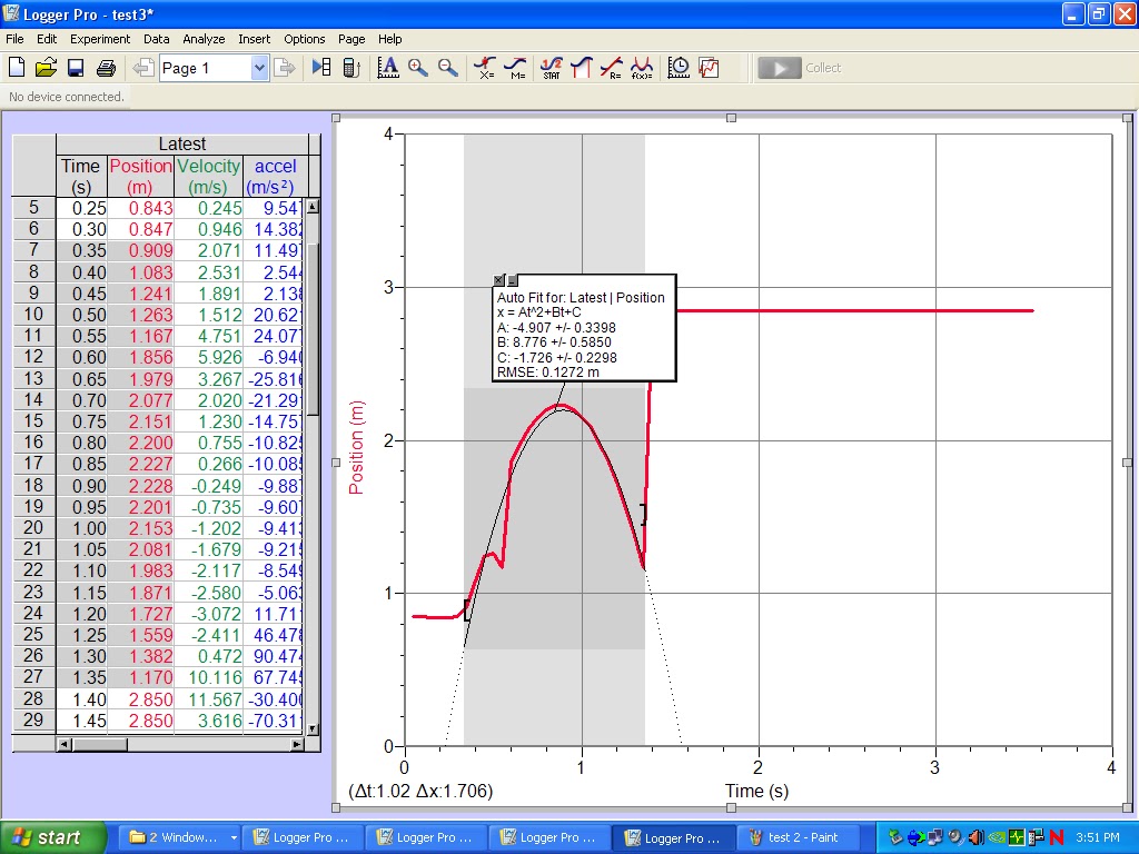
When doing this experiment and collecting data graphs, we expect to see the Position vs. Time graph to be a positive parabola because as time goes from 0 to

We did two linear fits on the velocity vs. time graph to obtain our a1 and a2. When finding a1, we did a linear fit when the velocity was moving at a constant rate less than 0 and for a2, we did a linear fit when the velocity was moving at a constant rate greater than 0. Those are going to make up our total average velocity that we used in the equation.

Trial 2:
We kept the set up the same but then we raised the incline to become steeper by adding another wood block underneath it. We measured out 50 cm on the track again and also used the level to make marks on the table vertically below the 0 cm and 50 cm mark to measure out the the length of the base of the "triangle" that the track and table make and that came to be 49.75 cm.

cosθ = (50cm/49.75cm)

arccos(cosθ) = arccos(50cm/49.75cm)

θ = 5.73°

Results:

Again, we took a linear fit of the negative velocity (a1) and the positive velocity (a2) that way we could take an average of the two for one average acceleration.

Conclusion:

In the first set of trials when we set the angle of the incline, θ, at 2.56°, our g-experimental value was 7.09 m/s^2. Our accepted value of g, g-accepted, is 9.80 m/s^2. With these numbers we can calculate a percent error that occurred  with the equation:

% error = |[(measured-actual)/actual]| X 100

=|[(7.09m/s^2 - 9.80m/s^2) / 9.8m/s^2]| X 100

=27.6%



Our second set of trials which ran on the elevated track were set at an angle θ = 5.73°. The average g-experimental value was 7.24 m/s^2. We can calculate the percent error:

|[(7.24m/s^2 - 9.8m/s^2) / 9.80m/s^2]| X 100

=26.1%

When we look at the position vs. time graphs of the cart in motion, we expect to see a positive parabola because as it starts traveling up the track it moves closer to the motion detector at a decreasing velocity which gives it a curve and not a line because the velocity is changing at a rate and not a constant. Once it gets to its highest point on the track, which is the closest point to the motion detector, the acceleration due to gravity takes over the cart and cart's position slowly starts to increase at a rate away from the motion detector which gives it an increasing curve. The graph would never have a negative position either because the cart approaches the motion detector which would have 0 position and once gravity takes over the carts velocity, the cart's position increases.

The velocity vs. time graph would be different though. It would be a line going in the positive direction that starts negative, crosses the x-axis which means it has velocity of 0 m/s at one point, and then becomes positive. This happens because the carts position is decreasing until it reaches its highest point as time increases which gives the cart negative velocity. The graph for velocity increases though since g is moving in the direction opposite direction until velocity reaches 0 m/s, which is the carts closest position to the motion detector. Then the velocity becomes positive because it starts increasing a changing rate as it travels in the same direction as acceleration and moves away from the motion detector increasing its position.

In this lab we observed the acceleration due to gravity of a cart as it travels up and inclined aluminum track as the velocity decreased and reached 0 m/s once the cart made it to its closest point to the motion detector and increased as the position increased. I learned how to calculate the acceleration due to gravity on an incline plane and showed the proof on how to find your experimental g. I also learned how to read and interpret the graphs such as the describing why the object has a parabolic position graph while it moves on the inclined plane and why the velocity graph is linear since the acceleration is constant. We had a large percent error when working with this lab but one major thing that could have contributed to the large error was that we could have taken a larger measurement when we were trying to find our angle of θ. We should have taken a larger measurerment of the track to find our angle because we could have gotten a more accurate measurement because there would have been a larger difference in our hypotenuse and the base leg of the triangle. I also think we had a lower percent error when we raised the angle of θ to be a bit higher also because the acceleration due to gravity could have more effect on the object since the plane is steeper.





Acceleration of Gravity Lab

We did this lab to serve to purposes: to determine the acceleration of gravity from a free falling object, and to gain experience using the computer software to collect data.

The materials needed for this lab are:

• a Lab Pro Interface
• Logger Pro Software on a computer
• Motion Detector
• rubber ball
• wire basket

In this lab we are trying to find the acceleration of gravity by measuring a the fall rubber ball with the motion detector hooked up to the Lab Pro Interface and collect the data onto Logger Pro where it will record it all. Logger Pro will also create a graph of both the velocity of the ball and the acceleration. We will look at these graphs to solve for the acceleration of gravity.

To begin this lab we loaded the Logger Pro software and opened the file, "graphlab", which contained the settings needed to run this lab. We are given a blank position vs. time graph which is where we will be collecting our data from. Set up the motion detector face up underneath the wire basket but in a space where none of the wires of the basket interfere with the motion detector. Also, make sure the motion detector is hooked up to the Lab Pro Interface, which also needs to be plugged into the computer's USB slot.
Once everything is hooked up and set, hit the "Collect" button, and throw the ball above the motion detector until it hits the ground and you see a position vs. time graph that has a negative quadratic parabola. We collected 5 of our best trials and saved their data. After we had the trials we wanted, we set a curve fit on all 5 position vs. time graphs to see what the equation would be that described the ball's motion of each trial. We solved for our experimental gravity for the trials (which is 2 times A, where A is the coefficient of the squared term of the equation given when you put on a curve fit) then solved for the percent error to show how close we were to solving for the accepted value for gravity, which is 9.8 (m/s)^2.
Change the y-axis label on the graph from position to velocity to show the velocity vs. time graph. Here, we want to find a part of the graph where there is a line to show a constant change in velocity with respect to time. Select the area that has the straightest line and select a linear fit in that portion of the graph. Do this to all 5 graphs and the slope, m, for all of these graphs should be close or equal to  -9.8 because the change in velocity describes acceleration. The constant change in velocity would show constant acceleration. Once solving for the value, m, calculate the % error and compare to your previous value for gravity.

CALCULATING PERCENT ERROR

percent error = |[(measured - actual)/actual]| X 100

DATA

This table shows our values of gravity compared to the accepted value for gravity as well as the percent error that occured for each graph.

GRAPHS 

TRIAL 1:

Position vs. Time

 

Velocity vs. Time

TRIAL 2:

Position vs. Time

Velocity vs. Time

TRIAL 3:
Position vs. Time

Velocity vs. Time

TRIAL 4:

Position vs. Time



Velocity vs. Time

TRIAL 5:
Position vs. Time

Velocity vs. Time



 

The graph of position is in the shape of a parabola because it is describing the distance of the ball from the motion detector. When the ball is first thrown, it's initial position is at about 1 m. Its height increases and time increases until it reaches it's highest point then it decreases in height falling at a faster pace the more time passes.

 

Each of these graphs all show the "A" value of their quadratic equations in the Position vs. Time graphs (in red). The slope, m, is given in the Velocity vs. Time graphs (in green) which describes the constant acceleration that occurs when the ball is thrown and is taken by gravity. The slope should be very close to -9.8 because that is acceleration of gravity.

 

The slope of the Velocity vs. Time graph represents the acceleration. When the velocity is positive it represents the increasing height of the ball. When it is equal to 0, this is when the ball reaches its heighest point and doesn't move for that split second. The negative velocity represents the ball falling from its highest point to when it hits the ground. The reason this graph is a line with a negative slope is because the as time increases, the slope of the position decreases from a positive slope to 0, then from 0 velocity down to a negative velocity.

Unit Analysis:

When we look at these graphs, we are given lots of information. When looking at the Position vs. Time Graphs for all of the trials you can see the equation of the fit that was performed. Looking at this equation we are given x=At^2+Bt+C where:

• A = acceleration.........................................(m/s^2)
• B = velocity................................................(m/s)
• C = position................................................(m)

You can solve for your experimental gravity by multiplying A by 2. It should be very close to if not -9.8 m/s^2. It is negative because gravity pulls things down which in mathematical terms means it is going in negative direction.

When looking at the graph of Velocity vs. Time we see something different. We see a line, not a parabola and instead of doing a curve fit we do a linear fit for this graph to find acceleration. Once performing a linear fit, you are given an equation v=mt+b where:

• m = acceleration...........................................(m/s^2)
• b = velocity..................................................(m/s)

We can use this graph to find our experimental gravity which in this case would be the m, or slope, of the velocity graph.

Conclusion:

In this lab, we looked at how to solve for the acceleration of gravity by tracking a falling ball and interpreting their Postion vs. Time graph as well as the Velocity vs. Time graph. I learned through the unit analysis, what each coefficient of quadratic and linear functions are and how they can help us solve for gravity. We were able to solve for the gravity from our results but they weren't all exactly the -9.80 m/s^2 we were trying to achieve. This is because of the errors that could have occured during lab like when we were throwing the ball there wasn't exactly a perfect scenario to make a perfect graph. Some things that could have possibly affected it was the motion detector not being able to follow the ball within 1 meter of it which made the graph do all the crazy spikes that occurred. That is why we ended up selecting a portion of the graph that was smooth and continuous to select a fit whether it was a curve fit or linear. There was also trial and error when throwing the ball up because we didn't get it perfectly above the motion sensor everytime and the motion detector was also covered by a wire basket that it could have picked up instead of the ball to throw our data off.